
Feature Importance
Feature importance의 개념 및 간단한 Python 실습 예제
안녕하세요, 태햄입니다.
첫 포스팅 주제는 Feature importance 입니다.
먼저 Feature importance 에 대한 개념을 이해하고 간단한 Python 실습을 통해 몸으로 익혀보도록 합시다 !
전반적인 내용은 이 곳 을 참고했습니다.
Feature importance란?
이 곳을 찾아오신 분이라면 한번 쯤 Data로부터 Feature를 뽑고 Machine learning (ML) 혹은 Deep Learning (DL)을 이용하여 모델을 구축하여 학습시킨 경험이 있으실텐데요, 이 과정에서 들었던 의문이 있으셨을 겁니다.
어떤 Feature가 이 모델에서 중요한 역할을 하는 Feature일까?
우리가 Model을 학습 시킬 때, Model에게 도움을 많이 줄 수 있는 Feature들만 최대한 확보하고 불필요한 정보는 학습에 사용하지 않는 것이 가장 현명한 방법이 되겠죠?
Feature importance 는 모델에 사용된 Feature들 중 모델의 학습에 기여한 정도에 따른 중요도 라고 할 수 있습니다.
특정 Feature가 모델의 정확도를 크게 높여준다면 이 Feature의 중요도 (importance) 또한 당연히 높겠죠?
Feature importance를 계산하는 방법은 모델에 따라 다양하지만, 오늘은 크게 세 가지를 소개해드리려고 합니다.
- Regression 에서 각 feature의 회귀 계수 (regression coefficient)를 이용한 방법
- 의사결정나무 (Decision Tree) 기반 분류 모델에서 불순도를 이용한 방법
- Permutation Feature importance
Feature importance를 통해 모델에 적절한 Feature들을 찾아 낼 수 있다면, 아래와 같은 기대효과를 얻을 수 있습니다.
- Data에 대한 더 깊은 이해
- Model에 대한 더 깊은 이해
- Input (Feature) 크기 축소 ( or 차원 축소 )
Scikit-Learn version 확인
본론에 들어가기 전에, 예제를 따라하시기 위해서 먼저 준비해야할 것들이 조금 있습니다.
Scikit-Learn 라이브러리를 이용하여 예제들을 진행할텐데, 버전을 확인하신 후 0.22.1 이상이 되도록 업데이트 해주시면 됩니다.
# Scikit-Learn Version check
import sklearn
print(sklearn.__version__)
0.24.1
버전이 0.22.1 미만이신분들은 아래와 같이 버전 업데이트를 해주시면 됩니다.
저는 업데이트를 해두어서 이미 0.24.1 버전으로 업그레이드가 되었다고 나오네요 ㅎㅎ
pip install --upgrade sklearn
Requirement already satisfied: sklearn in c:\users\imedisynrnd2\appdata\local\programs\python\python36\lib\site-packages (0.0)
Requirement already satisfied: scikit-learn in c:\users\imedisynrnd2\appdata\local\programs\python\python36\lib\site-packages (from sklearn) (0.24.1)
Requirement already satisfied: scipy>=0.19.1 in c:\users\imedisynrnd2\appdata\roaming\python\python36\site-packages (from scikit-learn->sklearn) (1.3.1)
Requirement already satisfied: joblib>=0.11 in c:\users\imedisynrnd2\appdata\local\programs\python\python36\lib\site-packages (from scikit-learn->sklearn) (0.14.0)
Requirement already satisfied: numpy>=1.13.3 in c:\users\imedisynrnd2\appdata\roaming\python\python36\site-packages (from scikit-learn->sklearn) (1.16.5)
Requirement already satisfied: threadpoolctl>=2.0.0 in c:\users\imedisynrnd2\appdata\local\programs\python\python36\lib\site-packages (from scikit-learn->sklearn) (2.1.0)
Note: you may need to restart the kernel to use updated packages.
Regression Feature Importance
Linear regression Model
먼저, make_regression() 함수를 이용해서 심플한 linear regression 모델에 쓰일 데이터를 생성해줍니다.
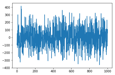
총 1000개의 샘플을 만들고, Feature 개수는 중요한 feature와 중요하지 않은 feature를 각각 5개씩 무작위로 생성해줍니다.
target data인 y를 그려보면 아래와 같이 생겼네요.
# Make regression dataset

from sklearn.datasets import make_regression
from sklearn.linear_model import LinearRegression

# Define dataset
X, y = make_regression(n_samples=1000, n_features=10, n_informative=5, random_state=1)

print(X.shape, y.shape) # size check

from matplotlib import pyplot
pyplot.plot(y)
pyplot.show()
(1000, 10) (1000,)
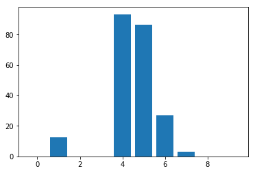
다음으로, model에 내장되어 있는 model.coef_ 함수를 통해 각 feature에 대한 회귀 계수 (regression coefficient)를 얻을 수 있습니다.
여기서 회귀 계수란, Linear Model $Y = b_{0} + b_{1}X_{1}+b_{2}X_{2}+ \cdots$ 에서 $b_{1}, b_{2} \cdots$ 에 해당하는 parameter를 말합니다.
이 회귀계수가 0과 가까울수록 모델에 대한 설명력이 없고, 0과 멀수록 모델에 대한 설명력이 강합니다.
아래 결과를 보면 총 10개의 Feature중 의미있는 5개의 Feature의 coefficient가 높게 나온 것을 확인할 수 있고, 이를 Importance로 사용한다면 중요한 Feature들 사이에서도 크기에 따라 importance의 순위를 매길 수도 있습니다.
# Define the model
model = LinearRegression()

# Fit the model
model.fit(X,y)

# Get importance
importance = model.coef_

# Summarize feature importance
for i,v in enumerate(importance):
    print('Feature: %0d, Score: %.5f' % (i,v))


from matplotlib import pyplot
# Plot feature importance
pyplot.bar([x for x in range(len(importance))], importance)
pyplot.show()
Feature: 0, Score: -0.00000
Feature: 1, Score: 12.44483
Feature: 2, Score: 0.00000
Feature: 3, Score: -0.00000
Feature: 4, Score: 93.32225
Feature: 5, Score: 86.50811
Feature: 6, Score: 26.74607
Feature: 7, Score: 3.28535
Feature: 8, Score: 0.00000
Feature: 9, Score: -0.00000
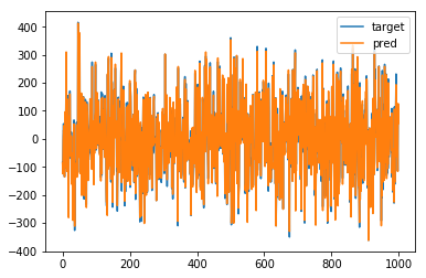
이 중에 중요한 5개의 Feature만 뽑아서 예측을 해보도록 하겠습니다. (1, 4, 5, 6, 7번 Feature)
아래와 같이 중요한 Feature만 뽑아서 써도 거의 정확하게 예측해내는 것을 볼 수 있습니다.
import numpy as np

select = [0,3,4,5,6]
pred = []

for i in range(1000):
    pred.append(np.dot(importance[select],X[i,select]))

pyplot.plot(y, label ='target')
pyplot.plot(pred, label = 'pred')
pyplot.legend()
pyplot.show()
Logistic regression Model
Logistic regression은 Binary Classification에 적용할 수 있는데요,
make_classification() 함수를 이용해서 logistic regression 모델에 쓰일 데이터를 생성해줍니다.
총 1000개의 샘플을 만들고, Feature 개수는 중요한 feature와 중요하지 않은 feature를 각각 5개씩 무작위로 생성해줍니다.
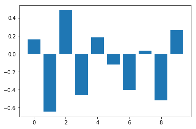
여기서도 역시 각 Feature들의 importance를 뽑고 비교해볼 수 있습니다.
# Logistic regression for reature importance
from sklearn.datasets import make_classification
from sklearn.linear_model import LogisticRegression
from matplotlib import pyplot

# Define dataset
X,y = make_classification(n_samples=1000, n_features=10, n_informative=5, n_redundant=5, random_state=1)

# Define the model
model = LogisticRegression()

# fit the model
model.fit(X, y)

# get importance
importance = model.coef_[0]

# Summarize feature importance
for i,v in enumerate(importance):
    print('Feature: %d, Score: %.5f' % (i,v))

# Plot feature importance
pyplot.bar([x for x in range(len(importance))], importance)
pyplot.show()
Feature: 0, Score: 0.16320
Feature: 1, Score: -0.64301
Feature: 2, Score: 0.48497
Feature: 3, Score: -0.46190
Feature: 4, Score: 0.18432
Feature: 5, Score: -0.11978
Feature: 6, Score: -0.40602
Feature: 7, Score: 0.03772
Feature: 8, Score: -0.51785
Feature: 9, Score: 0.26540
그렇다면, Logistic regression에서 중요한 feature들만 써서 예측을 해도 분류 성능이 유지될까요?
모든 feature들을 사용한 예측 결과와 feature importance가 높은 1, 2, 3, 6, 8 다섯개의 feature만 사용한 예측 결과를 비교해 보겠습니다.
# Use all features
model = LogisticRegression()
model.fit(X,y)
all_feature_pred = model.predict(X)
acc1 = np.mean(np.equal(y,all_feature_pred))*100

# Use five features
select = [0,1,2,5,7]
model2 = LogisticRegression()
model2.fit(X[:,select],y)
five_feature_pred = model2.predict(X[:,select])
acc2 = np.mean(np.equal(y,five_feature_pred))*100

import numpy as np
print('All feature accuracy : %.3f %% ' % acc1)
print('five feature accuracy : %.3f %%' % acc2)
All feature accuracy : 80.600 %
five feature accuracy : 80.500 %
간단한 Logistic regression 모델에서는 거의 차의가 없는 것을 알 수 있습니다.
성능 차이가 거의 없는데, feature 개수는 절반으로 줄었으니 굉장히 효율적이겠죠?
Decision Tree Feature Importance
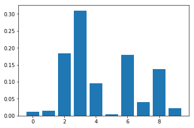
다음은 의사결정나무 (Decision Tree) 기반 모델의 Feature Importance입니다.
Decision Tree 기반 분류모델에서는 Feature Importance를 위해 불순도 (Impurity) 를 사용한다고 말씀드렸죠?
대표적으로 지니 계수 (Gini Index) 나 엔트로피 지수 (Entropy index) 를 사용합니다.
이와 관련된 자세한 내용은 Soo.P 님의 블로그에 자세히 정리되어 있으니 참고하시면 좋을 듯 합니다 :)
CART Classification Feature Importance
먼저, Decision Tree 기반 모델에서 유명한 CART (Classfication and Regression Tree) 알고리즘의 Feature Importance를 뽑아 보겠습니다. CART 알고리즘과 관련한 자세한 내용은 아래 링크들을 참고해 주세요 : )
Python은 대부분의 모델들을 이미 구축해서 라이브러리로 쉽게 이용할 수 있지만,
각 모델마다 조금씩 사용법이 다르니 검색해가시면서 사용하시면 됩니다 : )
CART를 위해 DecisionTreeClassifier 를 이용했구요, importance는 .feature_importance_ 를 이용하시면 됩니다.
# decision tree for feature importance on a classification problem
from sklearn.datasets import make_classification
from sklearn.tree import DecisionTreeClassifier
from matplotlib import pyplot

# define dataset
X, y = make_classification(n_samples=1000, n_features=10, n_informative=5, n_redundant=5, random_state=1)

# define the model
model = DecisionTreeClassifier()

# fit the model
model.fit(X, y)

# get importance
importance = model.feature_importances_

# summarize feature importance
for i,v in enumerate(importance):
 print('Feature: %0d, Score: %.5f' % (i,v))

# plot feature importance
pyplot.bar([x for x in range(len(importance))], importance)
pyplot.show()
Feature: 0, Score: 0.01131
Feature: 1, Score: 0.01496
Feature: 2, Score: 0.18424
Feature: 3, Score: 0.31016
Feature: 4, Score: 0.09518
Feature: 5, Score: 0.00400
Feature: 6, Score: 0.18000
Feature: 7, Score: 0.04073
Feature: 8, Score: 0.13772
Feature: 9, Score: 0.02171
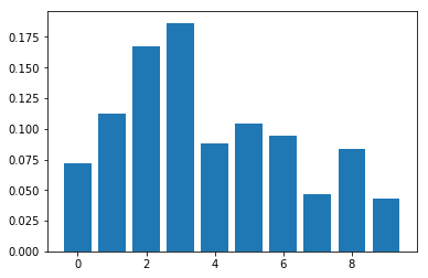
Random Forest Classification Feature Importance
Random forest에 대해서도 많이 들어보셨을 텐데요, Random forest는 여러개의 Decision Tree 모델을 병합하여 하나의 모델로 만드는 앙상블 (Emsemble) 기법 중 하나입니다. Regression과 Classification 모두 가능하지만 여기서는 Classification만 다뤄보도록 하겠습니다.
CART와 같은 방식으로 Feature Importance를 확인할 수 있습니다.
# random forest for feature importance on a classification problem
from sklearn.datasets import make_classification
from sklearn.ensemble import RandomForestClassifier
from matplotlib import pyplot

# define dataset
X, y = make_classification(n_samples=1000, n_features=10, n_informative=5, n_redundant=5, random_state=1)

# define the model
model = RandomForestClassifier()

# fit the model
model.fit(X, y)

# get importance
importance = model.feature_importances_

# summarize feature importance
for i,v in enumerate(importance):
 print('Feature: %0d, Score: %.5f' % (i,v))

# plot feature importance
pyplot.bar([x for x in range(len(importance))], importance)
pyplot.show()
Feature: 0, Score: 0.07224
Feature: 1, Score: 0.11277
Feature: 2, Score: 0.16749
Feature: 3, Score: 0.18646
Feature: 4, Score: 0.08850
Feature: 5, Score: 0.10417
Feature: 6, Score: 0.09475
Feature: 7, Score: 0.04685
Feature: 8, Score: 0.08381
Feature: 9, Score: 0.04296
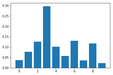
XGBoost Classification Feature Importance
최근 다양한 데이터 경진대회에서 각광을 받은 XGBoost (eXtream Gradient Boost) 입니다.
기존 Gradient Boost의 단점을 보완하여 유연한 parameter 조정이 가능하고 overfitting을 방지해주는 등 놀라운 성능을 보여주고 있죠.
역시 마찬가지로 Feature Importance를 뽑아 보겠습니다.
import warnings
warnings.filterwarnings("ignore")
warnings.simplefilter('ignore')

# xgboost for feature importance on a classification problem
from sklearn.datasets import make_classification
from xgboost import XGBClassifier
from matplotlib import pyplot


# define dataset
X, y = make_classification(n_samples=1000, n_features=10, n_informative=5, n_redundant=5, random_state=1)

# define the model
model = XGBClassifier()

# fit the model
model.fit(X, y)

# get importance
importance = model.feature_importances_

# summarize feature importance
for i,v in enumerate(importance):
    print('Feature: %0d, Score: %.5f' % (i,v))

# plot feature importance
pyplot.bar([x for x in range(len(importance))], importance)
pyplot.show()
Feature: 0, Score: 0.03723
Feature: 1, Score: 0.07725
Feature: 2, Score: 0.12537
Feature: 3, Score: 0.29666
Feature: 4, Score: 0.10099
Feature: 5, Score: 0.05706
Feature: 6, Score: 0.13027
Feature: 7, Score: 0.03537
Feature: 8, Score: 0.11694
Feature: 9, Score: 0.02285
Permutaion Feature Importance
Permutaion Feature importance는 어떤 모델이든 학습 시킨 후에, 특정 feature의 유무에 따른 성능의 차이를 확인할 수 있는 좋은 방법인데요!
장점을 정리하면 아래와 같습니다.
- 범용적이다 (어떤 모델이든 적용 가능하다)
- 계산이 빠르다 (학습을 시킨 후에 적용하므로)
- 특히, 불필요한 feature를 제거하는데 용이하다
자세한 내용은 아래 링크들을 참고해 주세요.
Python에서 제공하는 훌륭한 라이브러리인 eli5를 이용해서 Permutation Featire Importance를 뽑아 보려고 합니다. 마지막에 사용했던 모델인 XGBoost를 이용해보도록 하겠습니다.
import warnings
warnings.filterwarnings("ignore")
warnings.simplefilter('ignore')

# xgboost for feature importance on a classification problem
from sklearn.datasets import make_classification
from xgboost import XGBClassifier
from sklearn import metrics
from matplotlib import pyplot


# define dataset
X, y = make_classification(n_samples=1000, n_features=10, n_informative=5, n_redundant=5, random_state=1)

# define the model
model = XGBClassifier()

# fit the model
model.fit(X, y)

# get importance
importance = model.feature_importances_

import eli5
from eli5.sklearn import PermutationImportance

perm = PermutationImportance(model, random_state=1).fit(X,y)
eli5.show_weights(perm)
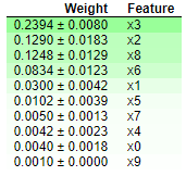
Permutaion Feature Importance를 이용했더니, 위에서 봤던 XGBoost의 Feature Importance 그래프와 동일한 내용이 표로 깔끔하게 정리된 것을 확인할 수 있습니다.
조금이라도 도움이 되셨길 바라며, 긴 글 읽어주셔서 감사드립니다.
다음에 또 다른 내용으로 찾아 뵙겠습니다 : )
Comments